CS131,Homewrok4,Resizing-SeamCarving
Seam Carving
The material presented here is inspired from:
- paper on seam carving: http://graphics.cs.cmu.edu/courses/15-463/2007_fall/hw/proj2/imret.pdf
- tutorial: http://cs.brown.edu/courses/cs129/results/proj3/taox
- tutorial: http://www.cs.cmu.edu/afs/andrew/scs/cs/15-463/f07/proj2/www/wwedler/
Don’t hesitate to check these links if you have any doubt on the seam carving process.
The whole seam carving process was covered in lecture 8, please refer to the slides for more details to the different concepts introduced here.
这份作业的主题是实现SeamCarving(接缝裁剪)的算法,即基于图像内容感知的图像缩放算法。
- 实现图像裁剪
- 实现图像扩大
- 其他实验
博客推荐
这篇专栏讲了如何用Python实现Seam carving算法,原理讲解的挺清楚的,看不懂英文可以看这个。
Sean Carving 的基本思路
- 计算图像能量图
- 寻找最小能量线
- 移除得到的最小能量线,让图片的宽度缩小一个像素
1 | # Setup |
The autoreload extension is already loaded. To reload it, use:
  %reload_ext autoreload
Image Reducing using Seam Carving
Seam carving is an algorithm for content-aware image resizing.
To understand all the concepts in this homework, make sure to read again the slides from lecture 8: http://vision.stanford.edu/teaching/cs131_fall1718/files/08_seam_carving.pdf
1 | from skimage import io, util |
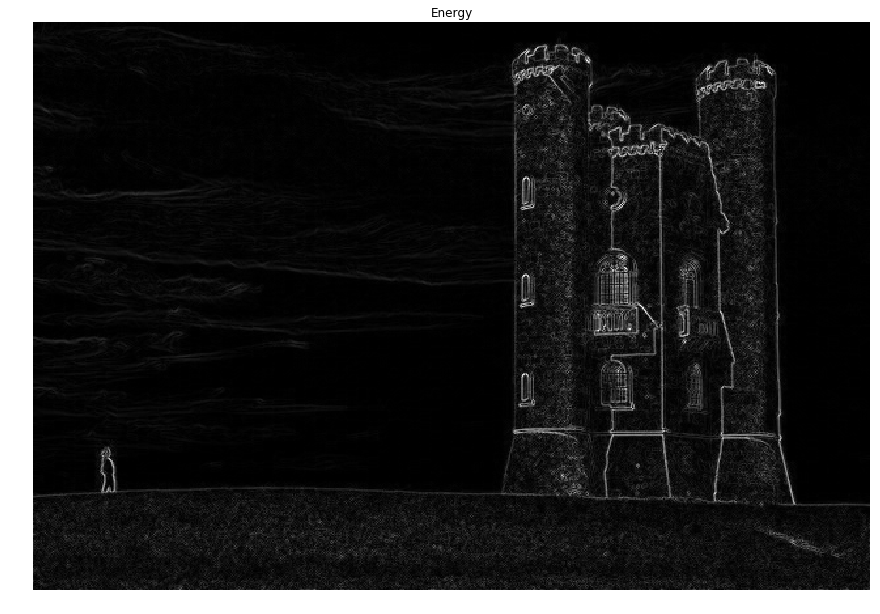
Energy function (5 points)
We will now implemented the energy_function to compute the energy of the image.
The energy at each pixel is the sum of:
- absolute value of the gradient in the $x$ direction
- absolute value of the gradient in the $y$ direction
The function should take around 0.01 to 0.1 seconds to compute.
图像能量图此处定义为图像每个像素的两方向梯度幅值之和,当然能量也可以是别的定义方式:梯度幅度、熵图、显著图等等。
计算梯度要注意转换为灰度图再进行。
1 | from seam_carving import energy_function |
Image (channel 0):
[[1.  2.  1.5]
 [3.  1.  2. ]
 [4.  0.5 3. ]]
Energy:
[[3.   1.25 1.  ]
 [3.5  1.25 1.75]
 [4.5  1.   3.5 ]]
Solution energy:
[[3.   1.25 1.  ]
 [3.5  1.25 1.75]
 [4.5  1.   3.5 ]]
1 | # Compute energy function |
Computing energy function: 0.007591 seconds.
跑出来的时间是0.009955 seconds,满足题目要求的0.01 to 0.1 seconds的时间范围。
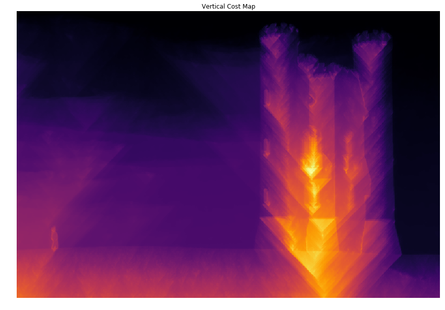
Compute cost (10 points)
Now implement the function compute_cost.
Starting from the energy map, we’ll go from the first row of the image to the bottom and compute the minimal cost at each pixel.
We’ll use dynamic programming to compute the cost line by line starting from the first row.
The function should take around 0.05 seconds to complete.
此处要求使用动态规划计算整幅图的cost图,用于第三步寻找最小能量线。
此处动态规划的意思是从图像的最上面一行开始,计算能量的最小累加路线,cost图中每一行的每个像素从它八相邻的上一行的三个像素中取最小cost值的元素进行累加。
直到累加到最后一行,同时在计算过程中保留每个像素的累加路径,即像素的cost值是从上一行哪一个元素相加得到的(用-1,0,1表示上左,上中,上右)。
题目中要求只用一个循环实现,则需要用向量化的形式进行计算。
1 | from seam_carving import compute_cost |
Energy:
[[1.  2.  1.5]
 [3.  1.  2. ]
 [4.  0.5 3. ]]
Cost:
[[1.  2.  1.5]
 [4.  2.  3.5]
 [6.  2.5 5. ]]
Solution cost:
[[1.  2.  1.5]
 [4.  2.  3.5]
 [6.  2.5 5. ]]
Paths:
[[ 0  0  0]
 [ 0 -1  0]
 [ 1  0 -1]]
Solution paths:
[[ 0  0  0]
 [ 0 -1  0]
 [ 1  0 -1]]
1 | # Vertical Cost Map |
Computing vertical cost map: 0.051953 seconds.
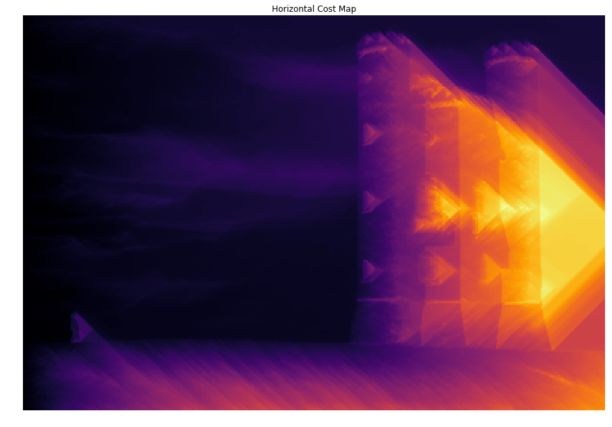
1 | # Horizontal Cost Map |
Computing horizontal cost map: 0.049583 seconds.
Finding optimal seams
Using the cost maps we found above, we can determine the seam with the lowest energy in the image.
We can then remove this optimal seam, and repeat the process until we obtain a desired width.
由于上面计算能量cost图时,已经保存了每个像素点的叠加路径,因此可以在最后一行找到最小的cost,并从该点开始,向上溯源,找到一条最佳的接缝,即最小的能量线。
Backtrack seam (5 points)
Implement function backtrack_seam.
1 | from seam_carving import backtrack_seam |
Seam Energy: 2.5
Seam: [0 1 1]
1 | vcost, vpaths = compute_cost(img, energy) |
Backtracking optimal seam: 0.000705 seconds.
Seam Energy: 2.443948431372548
到此,就实现了一条接缝的查找,接下来移除它就可以实现一个像素宽度的缩小。
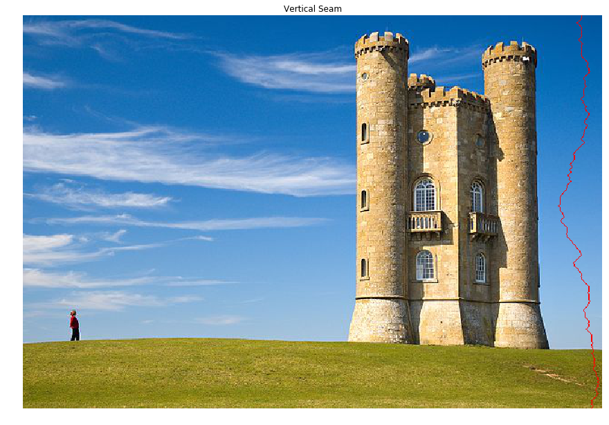
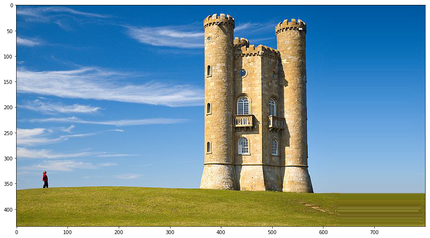
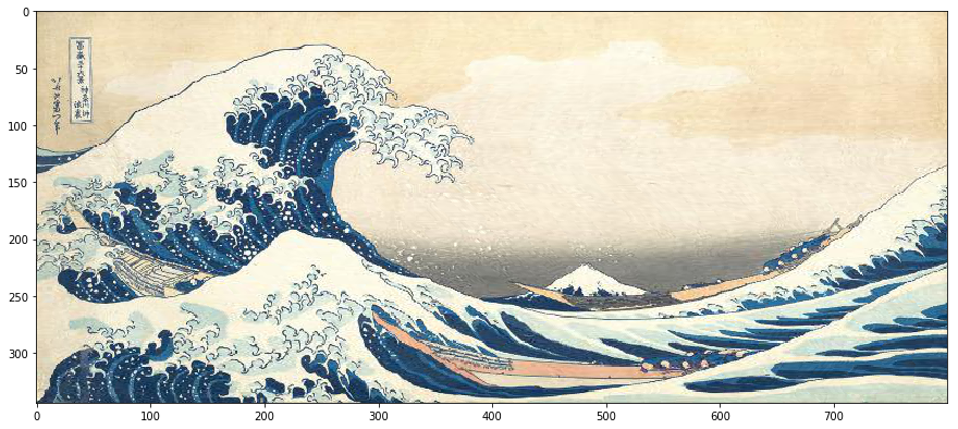
In the image above, the optimal vertical seam (minimal cost) goes through the portion of sky without any cloud, which yields the lowest energy.
Reduce (25 points)
We can now use the function backtrack and remove_seam iteratively to reduce the size of the image through seam carving.
Each reduce can take around 10 seconds to compute, depending on your implementation.
If it’s too long, try to vectorize your code in compute_cost to only use one loop.
1 | from seam_carving import reduce |
Original image (channel 0):
[[0. 1. 2.]
 [3. 4. 5.]
 [6. 7. 8.]]
Reduced image (channel 0): we see that seam [0, 4, 7] is removed
[[1. 2.]
 [3. 5.]
 [6. 8.]]
1 | # Reduce image width |
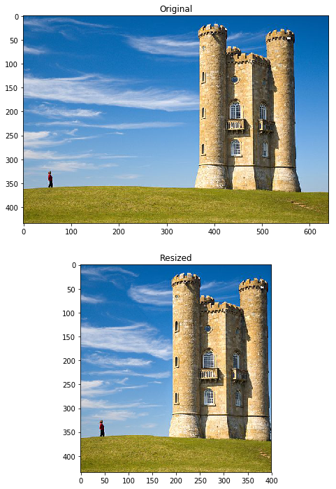
Reducing width from 640 to 400: 9.738185 seconds.
裁剪部分我是按照每一行删除一个元素的方式去实现的。
能够达到题目要求的10s左右的时间要求。
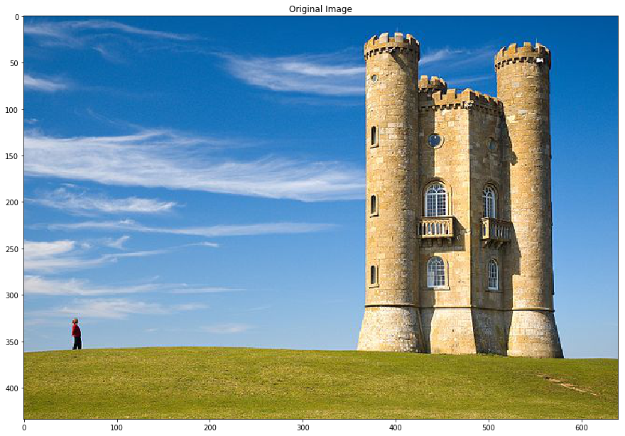
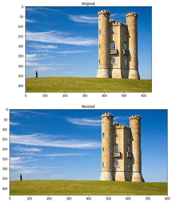
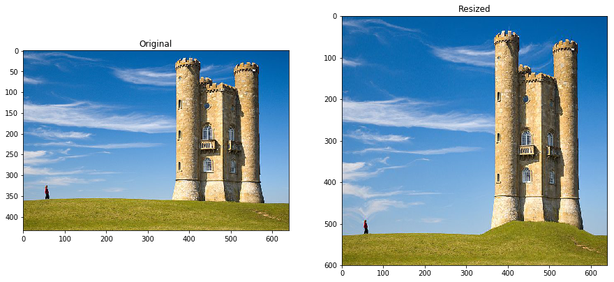
We observe that resizing from width 640 to width 400 conserves almost all the important part of the image (the person and the castle), where a standard resizing would have compressed everything.
All the vertical seams removed avoid the person and the castle.
程序同样可以缩减高度,程序中对于另一个维度的裁剪做了判断,
只需要seam carving流程走之前旋转图像,走完流程之后再将裁剪宽度的图像旋转回来就成了裁剪高度了。
1 | # Reduce image height |
Reducing height from 434 to 300: 7.296496 seconds.
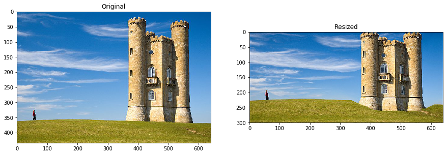
For reducing the height, we observe that the result does not look as nice.
The issue here is that the castle is on all the height of the image, so most horizontal seams will go through it.
Interestingly, we observe that most of the grass is not removed. This is because the grass has small variation between neighboring pixels (in a kind of noisy pattern) that make it high energy.
The seams removed go through the sky on the left, go under the castle to remove some grass and then back up in the low energy blue sky.
虽然实现了高度的裁剪,但是图像看起来怪怪的,这是可以从图像上做分析的。
城堡明显具有很强的能量,详见第一步能量图计算,因此裁剪高度时,每一条最小能量线都会越过它。
草坪看起来其实跟噪声一样,每个像素点与相邻像素都有或大或小的差异,因此梯度也是较大的,因此能量也较高,不会首先裁剪草坪而是更平滑的蓝天,
而城堡下面的草坪凹陷是因为城堡上方的蓝天已被裁剪光了,最小能量线无法从上方穿过时才从城堡下方的草坪开始裁剪的。
Image Enlarging
Enlarge naive (10 points)
We now want to tackle the reverse problem of enlarging an image.
One naive way to approach the problem would be to duplicate the optimal seam iteratively until we reach the desired size.
图像扩大的一种方式是直接在最小能量线的地方复制它。
在enlarge_naive函数中实现它。
1 | from seam_carving import enlarge_naive |
Original image (channel 0):
[[0. 1. 2.]
 [3. 4. 5.]
 [6. 7. 8.]]
Enlarged image (channel 0): we see that seam [0, 4, 7] is duplicated
[[0. 0. 1. 2.]
 [3. 4. 4. 5.]
 [6. 7. 7. 8.]]
1 | W_new = 800 |
Enlarging(naive) height from 640 to 800: 8.824498 seconds.
The issue with enlarge_naive is that the same seam will be selected again and again, so this low energy seam will be the only to be duplicated.
Another way to get k different seams is to apply the process we used in function reduce, and keeping track of the seams we delete progressively.
The function find_seams(image, k) will find the top k seams for removal iteratively.
The inner workings of the function are a bit tricky so we’ve implemented it for you, but you should go into the code and understand how it works.
This should also help you for the implementation of enlarge.
直接复制的方式明显有问题:在最小能量线的地方不停的迭代复制(复制同一个地方),会造成该区域的不自然。
作业已经帮忙实现了:查找k条不同的接缝,这样就可以根据k条接缝来轮流进行删除了。
1 | from seam_carving import find_seams |
Finding 160 seams: 7.296915 seconds.
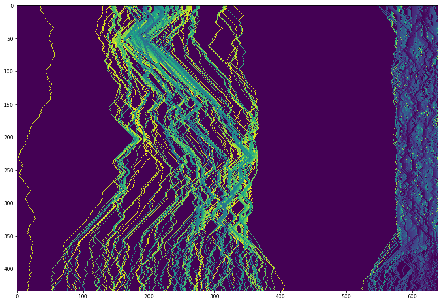
不同的颜色是因为按照排序,给每条路线的标记的值不同。
Enlarge (25 points)
We can see that all the seams found are different, and they avoid the castle and the person.
One issue we can mention is that we cannot enlarge more than we can reduce. Because of our process, the maximum enlargement is the width of the image W because we first need to find W different seams in the image.
One effect we can see on this image is that the blue sky at the right of the castle can only be enlarged x2. The concentration of seams in this area is very strong.
We can also note that the seams at the right of the castle have a blue color, which means they have low value and were removed in priority in the seam selection process.
值得注意的是,对于图像能放大的像素宽度肯定不会超过图像能缩减的像素宽度,毕竟最小能量线就只有那么多条。
实现enlarge函数。
1 | from seam_carving import enlarge |
Original image (channel 0):
[[0. 1. 3.]
 [0. 1. 3.]
 [0. 1. 3.]]
Enlarged naive image (channel 0): first seam is duplicated twice.
[[0. 0. 0. 1. 3.]
 [0. 0. 0. 1. 3.]
 [0. 0. 0. 1. 3.]]
Enlarged image (channel 0): first and second seam are each duplicated once.
[[0. 0. 1. 1. 3.]
 [0. 0. 1. 1. 3.]
 [0. 0. 1. 1. 3.]]
1 | W_new = 800 |
Enlarging width from 640 to 800: 10.235673 seconds.
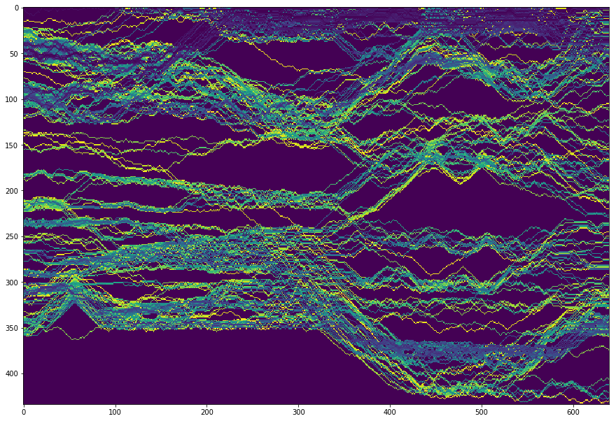
1 | # Map of the seams for horizontal seams. |
Finding 160 seams: 9.089754 seconds.
1 | H_new = 600 |
Enlarging height from 434 to 600: 14.027314 seconds.
As you can see in the example above, the sky above the castle has doubled in size, the grass below has doubled in size but we still can’t reach a height of 600.
The algorithm then needs to enlarge the castle itself, while trying to avoid enlarging the windows for instance.
Other experiments on the image
Feel free to experiment more on this image, try different sizes to enlarge or reduce, or check what seams are chosen…
Reducing by a 2x factor often leads to weird patterns.
Enlarging by more than 2x is impossible since we only duplicate seams. One solution is to enlarge in mutliple steps (enlarge x1.4, enlarge again x1.4…)
放大两倍或者缩小二分之一图像会变得很奇怪。
这里提出一个方式就是进行多次Resize步骤,每次x1.4倍,x1.4倍这样的方式来放大,缩小同理。
1 | # Reduce image width |
Reducing width from 640 to 200: 16.882833 seconds.

Faster reduce (extra credit 0.5%)
Implement a faster version of reduce called reduce_fast in the file seam_carving.py.
We will have a leaderboard on gradescope with the performance of students.
The autograder tests will check that the outputs match, and run the reduce_fast function on a set of images with varying shapes (say between 200 and 800).
思路
怎么能实现更快地裁剪呢?
题目的提示是:do we really need to compute the whole cost map again at each iteration?
分析了一下reduce的过程,的确有一块是可以改进的。
1 | while out.shape[1] > size: |
就是计算energy能量图这一步,因为能量图的计算其实就是梯度的计算。
如果一个区域内的图像像素不变动的话,那这个区域内的梯度应该也不会放生改变,基于这一点,可以对计算能量图的步骤进行改进。
只需要对上一次optical seam最小能量线覆盖宽度内的区域进行梯度的重新更新,两侧区域的能量值不需要变动。
比如接缝最左边为left,则left-1处像素不变,梯度改变,left-2处及之前像素不变梯度不变。
比如接缝最右边为right,则right+1处像素不变,梯度改变,left+2处及之后像素不变梯度不变。
然后考虑特殊情况。
1 | from seam_carving import reduce_fast |
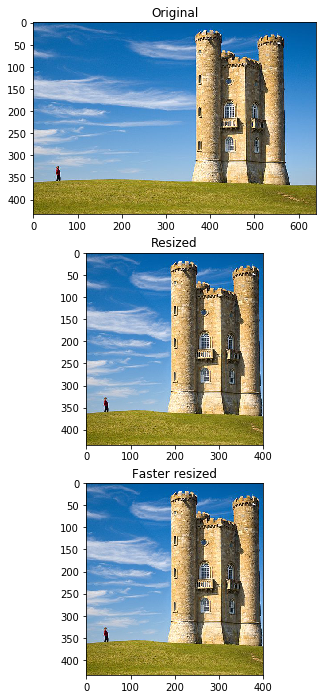
Normal reduce width from 640 to 400: 9.237779 seconds.
Faster reduce width from 640 to 400: 8.685472 seconds.
Reducing and enlarging on another image
Also check these outputs with another image.
1 | # Load image |
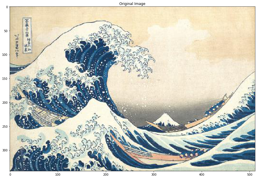
1 | out = reduce(img2, 300) |
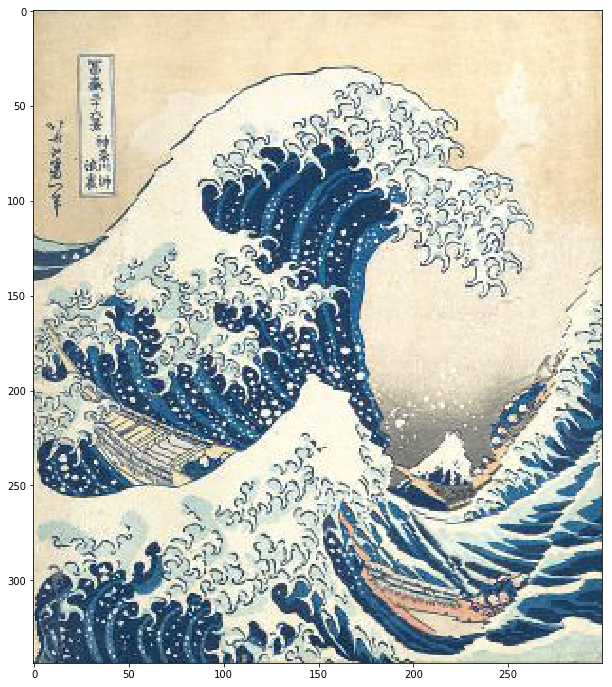
1 | out = enlarge(img2, 800) |
Forward Energy (20 points)
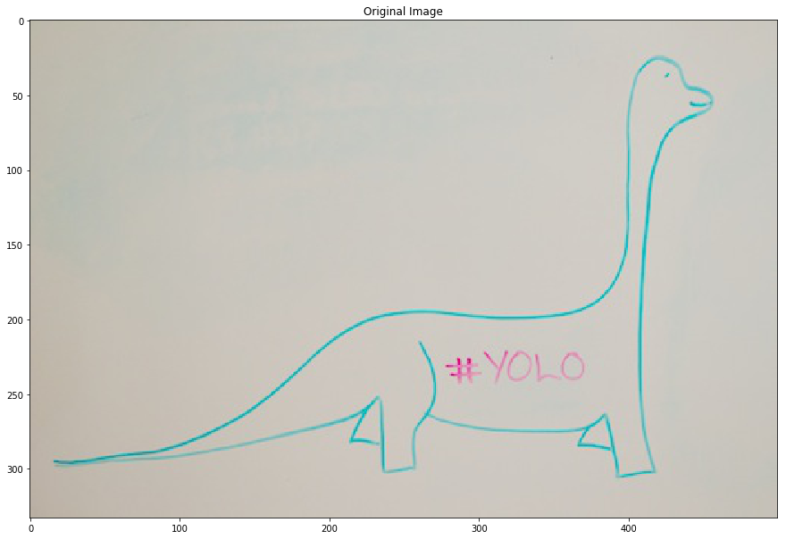
Forward energy is a solution to some artifacts that appear when images have curves for instance.
Implement the function compute_forward_cost. This function will replace the compute_cost we have been using until now.
基本的seam carving 会影响物体的原有结构,比如曲线啊。
因此提出了Forward Energy这个方法。
详见 CS131 Lecture8 的PPT P76-P86。
介绍上说的是 Instead of removing the seam of least energy, remove the seam that inserts the least energy to the image !
之前的做法是去除掉具有最小能量的接缝,而Forward Energy的做法是去除掉给整张图像带来最小能量的接缝。
具体的可视化解释在PPT中,这里就放公式了。
之前的能量图定义为
$$ M(i,j) = E(i,j) + min \left\{ \begin{array}{lr} M(i-1,j-1) \\ M(i-1,j) \\ M(i-1,j+1) \end{array} \right. $$Forward能量图的定义为
$$ M(i,j) = E(i,j) + min \left\{ \begin{array}{lr} M(i-1,j-1) + C_L(i,j), & C_L(i,j) = |I(i,j+1) - I(i,j-1)| + |I(i-1,j) - I(i,j-1)|\\ M(i-1,j) + C_V(i,j), & C_V(i,j) = |I(i,j+1) - I(i,j-1)| \\ M(i-1,j+1)+C_R(i,j), , & C_R(i,j) = |I(i,j+1) - I(i,j-1)| + |I(i-1,j) - I(i,j+1)|\ \end{array} \right. $$1 | # Load image |
1 | from seam_carving import compute_forward_cost |
Image:
[[1.  1.  2. ]
 [0.5 0.  0. ]
 [1.  0.5 2. ]]
Energy:
[[0.5 1.5 3. ]
 [0.5 0.5 0. ]
 [1.  1.  3.5]]
Cost:
[[0.5 2.5 3. ]
 [1.  2.  3. ]
 [2.  4.  6. ]]
Solution cost:
[[0.5 2.5 3. ]
 [1.  2.  3. ]
 [2.  4.  6. ]]
Paths:
[[ 0  0  0]
 [ 0 -1  0]
 [ 0 -1 -1]]
Solution paths:
[[ 0  0  0]
 [ 0 -1  0]
 [ 0 -1 -1]]
1 | from seam_carving import compute_forward_cost |
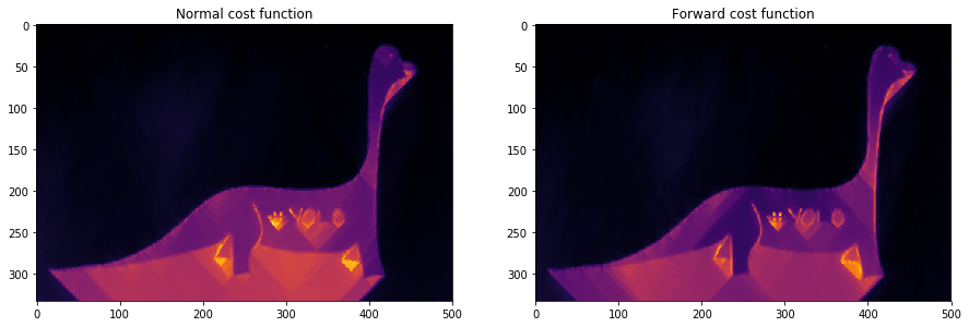
We observe that the forward energy insists more on the curved edges of the image.
可以看到,Forward Energy方法在保留边缘曲线的结构上比原方法好。
1 | from seam_carving import reduce |
Old Solution: 5.034606 seconds.

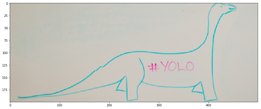
The issue with our standard reduce function is that it removes vertical seams without any concern for the energy introduced in the image.
In the case of the dinosaure above, the continuity of the shape is broken. The head is totally wrong for instance, and the back of the dinosaure lacks continuity.
Forward energy will solve this issue by explicitely putting high energy on a seam that breaks this continuity and introduces energy.
1 | # This step can take a very long time depending on your implementation. |
Forward Energy Solution: 8.092415 seconds.
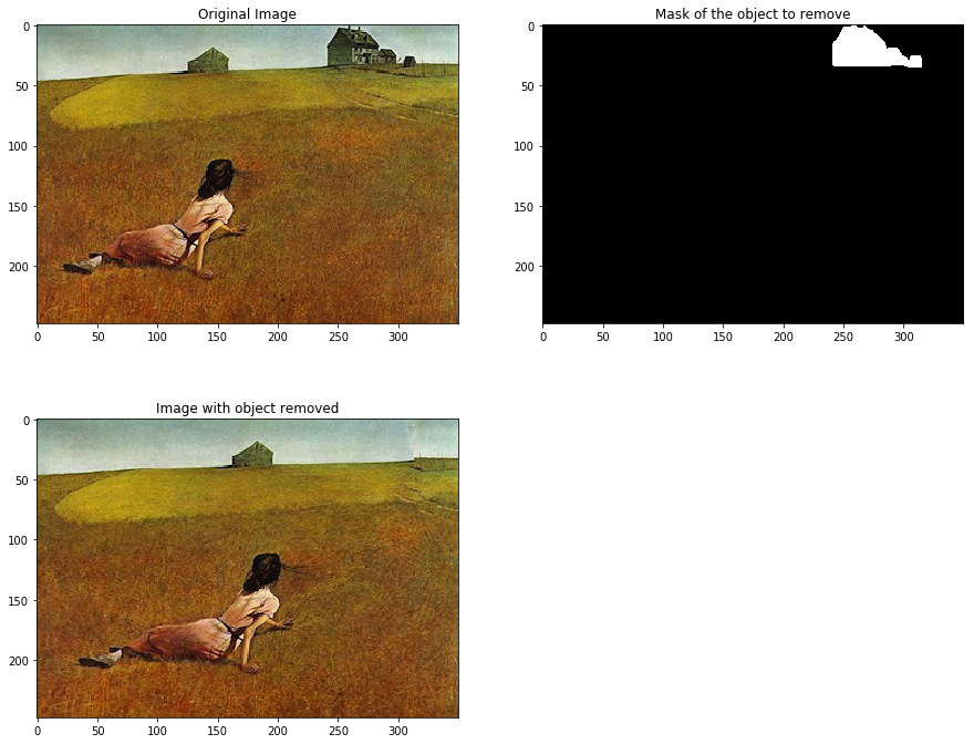
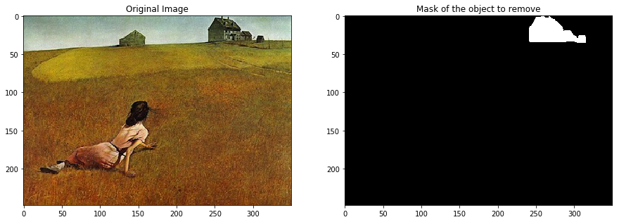
Object removal (extra credit 0.5%)
Object removal uses a binary mask of the object to be removed.
Using the reduce and enlarge functions you wrote before, complete the function remove_object to output an image of the same shape but without the object to remove.
移除目标和保留目标
移除目标的思路应该很清晰,就是将图像中目标处的像素视为能量最小或最大,即可将目标去除了。
两个问题:
- 如何进行标记,从而每次删除能量线的时候,都能删到并且尽可能多的删到带有标记的能量线?同时坐标下标不会混乱。
- 如何在删除目标之后保持和原图同样的尺寸
解决方式也不难:
- 判断最小能量线的时候,将mask区域乘上负数,自然找到的接缝能量会最小,并且穿过mask区域的像素点会更多。
- 做裁剪的时候,将mask根据接缝和图像一起进行裁剪,自然不会引起下标混乱。
- 删除目标之后再调用之前的enlarge函数,进行图像的放大,放大到原图尺寸。
1 | # Load image |
/home/ubuntu/anaconda3/lib/python3.6/site-packages/skimage/util/dtype.py:118: UserWarning: Possible sign loss when converting negative image of type float64 to positive image of type bool.
  .format(dtypeobj_in, dtypeobj_out))
/home/ubuntu/anaconda3/lib/python3.6/site-packages/skimage/util/dtype.py:122: UserWarning: Possible precision loss when converting from float64 to bool
  .format(dtypeobj_in, dtypeobj_out))
1 | # Use your function to remove the object |