CS131, Homewrok2, Edges-Smart Car Lane Detection
Homework 2
This notebook includes both coding and written questions. Please hand in this notebook file with all the outputs and your answers to the written questions.
这份作业的知识点包括边缘检测(实现Canny 边缘检测算子)和霍夫变换。
1 | # Setup |
The autoreload extension is already loaded. To reload it, use:
  %reload_ext autoreload
Part 1: Canny Edge Detector (85 points)
In this part, you are going to implment Canny edge detector. The Canny edge detection algorithm can be broken down in to five steps:
- Smoothing:平滑处理(去躁)
- Finding gradients:寻找梯度
- Non-maximum suppression:非极大值抑制
- Double thresholding:双阈值算法
- Edge tracking by hysteresis:滞后边缘追踪
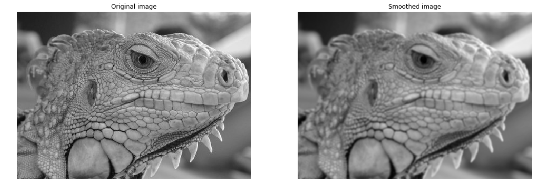
1.1 Smoothing (10 points)
Implementation (5 points)
We first smooth the input image by convolving it with a Gaussian kernel. The equation for a Gaussian kernel of size $(2k+1)\times(2k+1)$ is given by:
$$
h_{ij}=\frac{1}{2\pi\sigma^2}\exp{\Bigl(-\frac{(i-k)^2+(j-k)^2}{2\sigma^2}\Bigr)}, 0\leq i,j < 2k+1
$$
Implement gaussian_kernel in edge.py and run the code below.
代码实现高斯核的生成。
1 | from edge import conv, gaussian_kernel |
需要先实现edge.py中的conv卷积函数,可以使用作业hw1中的conv_nested,conv_fast,conv_faster等函数
1 | # Test with different kernel_size and sigma |
Question (5 points)
What is the effect of the kernel_size and sigma?
kernel_size和标准差 $\sigma$ 的影响?
Your Answer: Write your solution in this markdown cell.
高斯滤波器用像素邻域的加权均值来代替该点的像素值,而每一邻域像素点权值是随该点与中心点的距离单调增减的,因为边缘是一种图像局部特征,如果平滑运算对离算子中心很远的像素点仍然有很大作用,则平滑运算会使图像失真。
高斯滤波器宽度(决定着平滑程度)是由参数σ表征的,而且σ和平滑程度的关系是非常简单的.σ越大,高斯滤波器的频带就越宽,平滑程度就越好.通过调节平滑程度参数σ,可在图像特征过分模糊(过平滑)与平滑图像中由于噪声和细纹理所引起的过多的不希望突变量(欠平滑)之间取得折衷。
参考:高斯噪声与高斯滤波
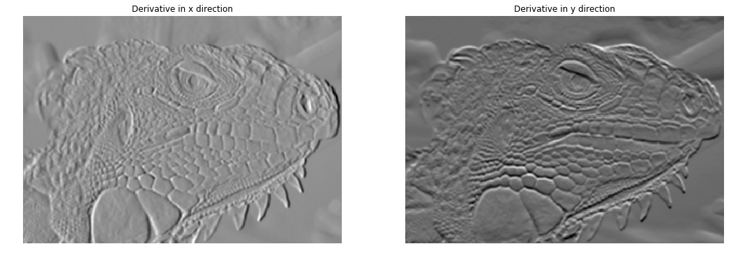
1.2 Finding gradients (15 points)
The gradient of a 2D scalar function $I:\mathbb{R}^2\rightarrow{\mathbb{R}}$ in Cartesian coordinate is defined by:
$$
\nabla{I(x,y)}=\bigl[\frac{\partial{I}}{\partial{x}},\frac{\partial{I}}{\partial{y}}\bigr],
$$
where
$$
\frac{\partial{I(x,y)}}{\partial{x}}=\lim_{\Delta{x}\to{0}}\frac{I(x+\Delta{x},y)-I(x,y)}{\Delta{x}} \
\frac{\partial{I(x,y)}}{\partial{y}}=\lim_{\Delta{y}\to{0}}\frac{I(x,y+\Delta{y})-I(x,y)}{\Delta{y}}.
$$
In case of images, we can approximate the partial derivatives by taking differences at one pixel intervals:
$$
\frac{\partial{I(x,y)}}{\partial{x}}\approx{\frac{I(x+1,y)-I(x-1,y)}{2}} \
\frac{\partial{I(x,y)}}{\partial{y}}\approx{\frac{I(x,y+1)-I(x,y-1)}{2}}
$$
Note that the partial derivatives can be computed by convolving the image $I$ with some appropriate kernels $D_x$ and $D_y$:
$$ \frac{\partial{I}}{\partial{x}}\approx{I*D_x}=G_x \\ \frac{\partial{I}}{\partial{y}}\approx{I*D_y}=G_y $$Implementation (5 points)
Find the kernels $D_x$ and $D_y$ and implement partial_x and partial_y using conv defined in edge.py.
-Hint: Remeber that convolution flips the kernel.
实现edge.py中的partial_x和partial_y函数
1 | from edge import partial_x, partial_y |
1 | # Compute partial derivatives of smoothed image |
Question (5 points)
What is the reason for performing smoothing prior to computing the gradients?
梯度计算前为何要进行平滑滤波?
Your Answer: Write your solution in this markdown cell.
答
平滑是为了去噪,噪声会使得计算梯度时得到幅度较大的异常值。
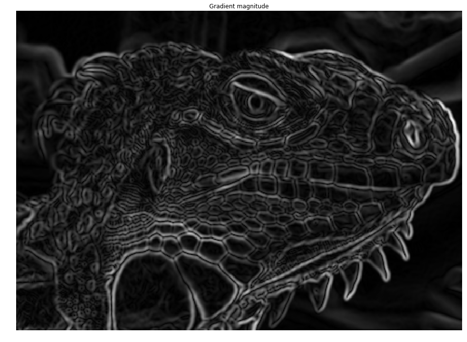
Implementation (5 points)
Now, we can compute the magnitude and direction of gradient with the two partial derivatives:
$$
G = \sqrt{G_{x}^{2}+G_{y}^{2}} \
\Theta = arctan\bigl(\frac{G_{y}}{G_{x}}\bigr)
$$
Implement gradient in edge.py which takes in an image and outputs $G$ and $\Theta$.
-Hint: Use np.arctan2 to compute $\Theta$.
1 | from edge import gradient |
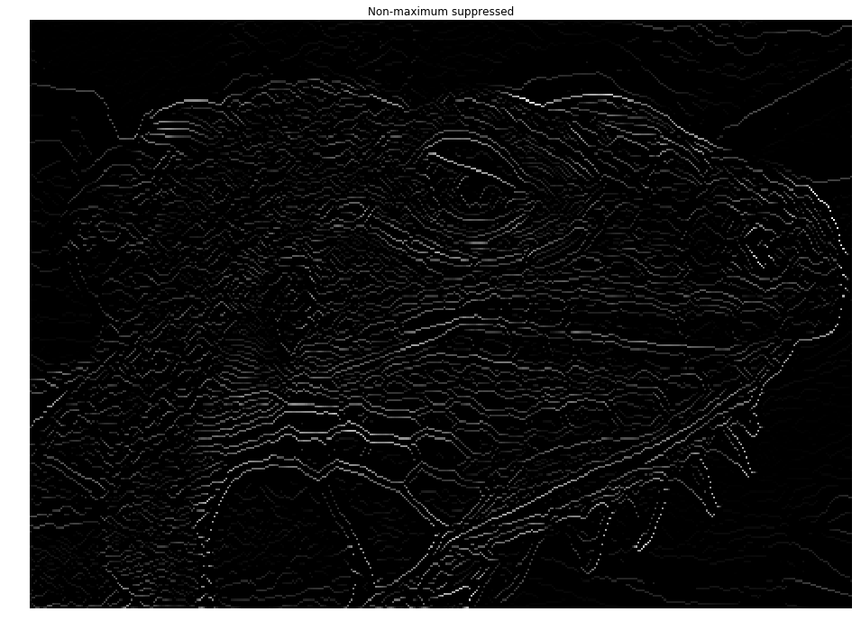
1.3 Non-maximum suppression (15 points)
You should be able to note that the edges extracted from the gradient of the smoothed image is quite thick and blurry. The purpose of this step is to convert the “blurred” edges into “sharp” edges. Basically, this is done by preserving all local maxima in the gradient image and discarding everything else. The algorithm is for each pixel (x,y) in the gradient image:
Round the gradient direction $\Theta[y,x]$ to the nearest 45 degrees, corresponding to the use of an 8-connected neighbourhood.
Compare the edge strength of the current pixel with the edge strength of the pixel in the positive and negative gradient direction. For example, if the gradient direction is south (theta=90), compare with the pixels to the north and south.
If the edge strength of the current pixel is the largest; preserve the value of the edge strength. If not, suppress (i.e. remove) the value.
Implement non_maximum_suppression in edge.py
非极大值抑制属于一种边缘细化的方法,梯度大的位置有可能为边缘,在这些位置沿着梯度方向,找到像素点的局部最大值,并将其非最大值抑制。
形象的说就是一条粗粗的区域都根据梯度强度判断成了边缘,但目标只需要一条细细的边,这个时候就找区域内的最大的那条作为边(注意是沿着梯度方向),其他的或抛弃或作为备选区域
步骤
- 在0,45,90,135四个梯度方向上对8-邻接像素进行判断,
- 直接比较梯度方向上的相邻的两个像素,
- 如果当前像素强度是最大,则保留;否则,则抑制它(变为零)。
备注
当然这种做法其实是简化版本的,虽然Canny的论文上是这么写的,但是后来也有提出,梯度肯定不止这四个,针对别的梯度方向的比较,使用插值等方法来进行非极大值抑制。
可以参考:Canny算子中的非极大值抑制(Non-Maximum Suppression)分析
1 | from edge import non_maximum_suppression |
Thetas: 0
[[0.  0.  0.6]
 [0.  0.  0.7]
 [0.  0.  0.6]]
Thetas: 45
[[0.4 0.5 0.6]
 [0.  0.  0.7]
 [0.  0.  0.6]]
Thetas: 90
[[0.4 0.5 0. ]
 [0.  0.5 0.7]
 [0.4 0.5 0. ]]
Thetas: 135
[[0.  0.  0.6]
 [0.  0.  0.7]
 [0.4 0.5 0.6]]
目测是正确的。在每个梯度方向上保留最大的那个值,其他的值置为零。
1 | nms = non_maximum_suppression(G, theta) |
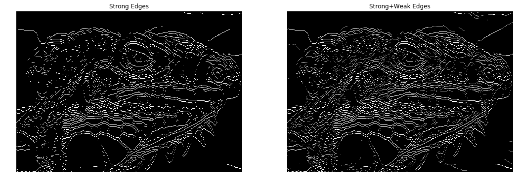
1.4 Double Thresholding (20 points)
The edge-pixels remaining after the non-maximum suppression step are (still) marked with their strength pixel-by-pixel. Many of these will probably be true edges in the image, but some may be caused by noise or color variations, for instance, due to rough surfaces. The simplest way to discern between these would be to use a threshold, so that only edges stronger that a certain value would be preserved. The Canny edge detection algorithm uses double thresholding. Edge pixels stronger than the high threshold are marked as strong; edge pixels weaker than the low threshold are suppressed and edge pixels between the two thresholds are marked as weak.
Implement double_thresholding in edge.py
双阀值方法,设置一个maxval,以及minval,梯度大于maxval则为强边缘,梯度值介于maxval与minval则为弱边缘点,小于minval为抑制点。
双阈值的结果在第五步可以用来作为边缘追踪的依据。
1 | from edge import double_thresholding |
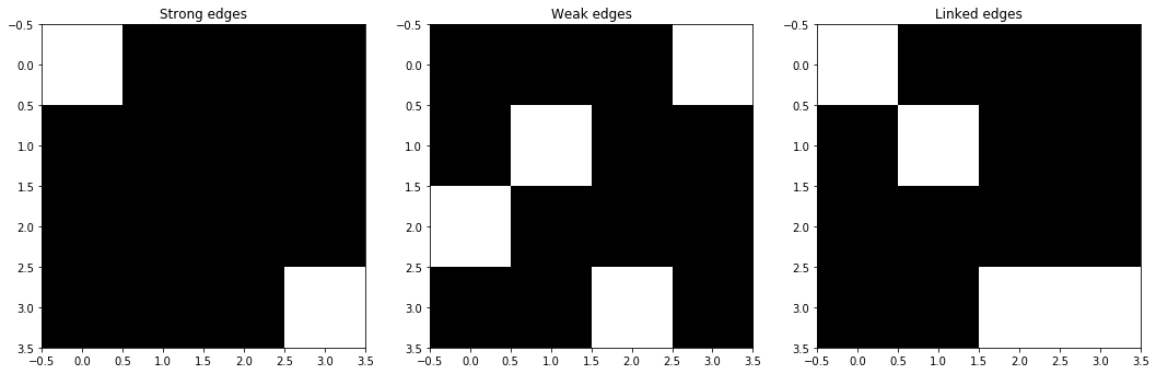
1.5 Edge tracking (15 points)
Strong edges are interpreted as “certain edges”, and can immediately be included in the final edge image. Weak edges are included if and only if they are connected to strong edges. The logic is of course that noise and other small variations are unlikely to result in a strong edge (with proper adjustment of the threshold levels). Thus strong edges will (almost) only be due to true edges in the original image. The weak edges can either be due to true edges or noise/color variations. The latter type will probably be distributed in dependently of edges on the entire image, and thus only a small amount will be located adjacent to strong edges. Weak edges due to true edges are much more likely to be connected directly to strong edges.
Implement link_edges in edge.py
由于边缘是连续的,因此可以认为弱边缘如果为真实边缘则和强边缘是联通的,可由此判断其是否为真实边缘。
1 | from edge import get_neighbors, link_edges |
1 | edges = link_edges(strong_edges, weak_edges) |
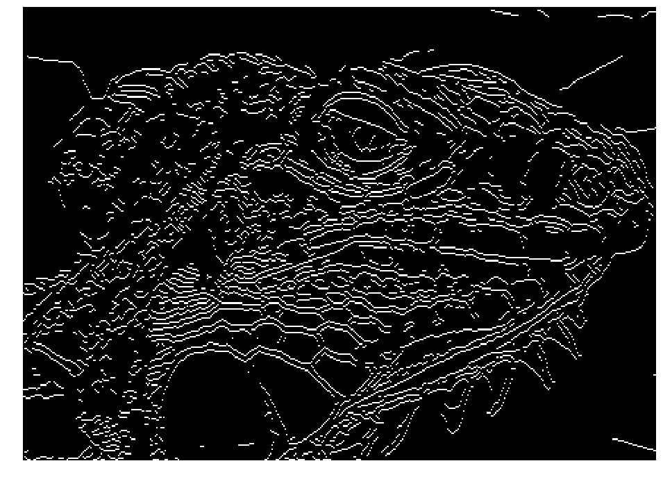
1.6 Canny edge detector
Implement canny in edge.py using the functions you have implemented so far. Test edge detector with different parameters.
Here is an example of the output:

将上面的五个步骤拼成一个Canny边缘检测算子。
- Smoothing:平滑处理(去躁)
- Finding gradients:寻找梯度
- Non-maximum suppression:非极大值抑制
- Double thresholding:双阈值算法
- Edge tracking by hysteresis:滞后边缘追踪
1 | from edge import canny |
(310, 433)
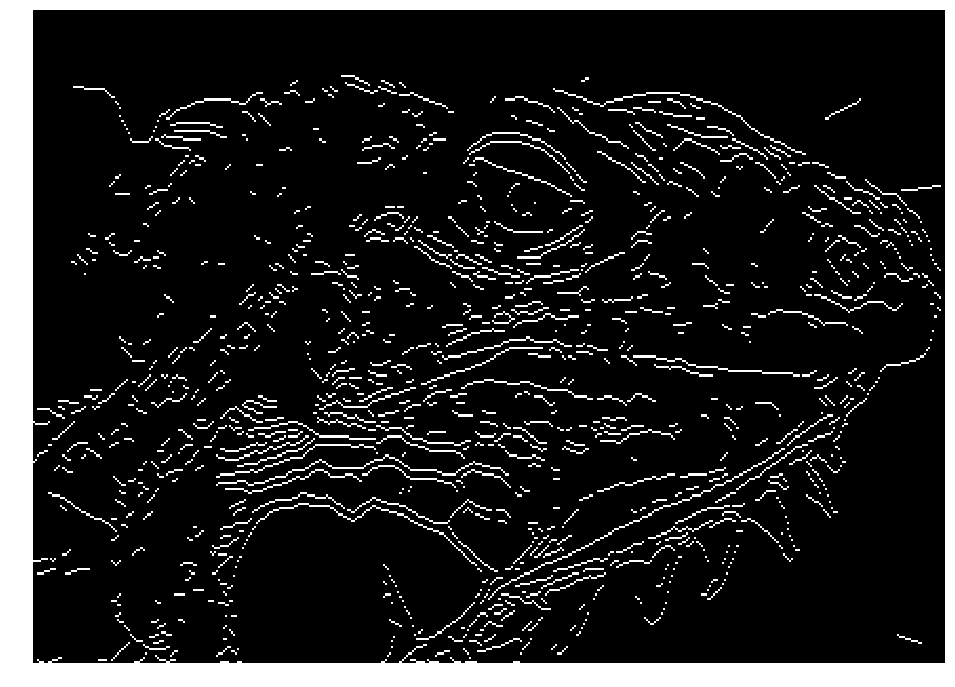
怎么调参也调不出合理的效果,应该是此时非极大值抑制,抑制的有些过分了。
1.7 Question (10 points)
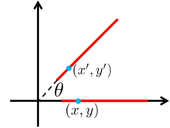
(a) Suppose that the Canny edge detector successfully detects an edge in an image. The edge (see the figure above) is then rotated by θ, where the relationship between a point on the original edge $(x, y)$ and a point on the rotated edge $(x’, y’)$ is defined as
$$
x’=x\cos{\theta}\
y’=x\sin{\theta}
$$
Will the rotated edge be detected using the same Canny edge detector? Provide either a mathematical proof or a counter example.
-Hint: The detection of an edge by the Canny edge detector depends only on the magnitude of its derivative. The derivative at point (x, y) is determined by its components along the x and y directions. Think about how these magnitudes have changed because of the rotation.
Your Answer: Write your solution in this markdown cell.
$$ Mag_{origin} = \sqrt {{dx}^2 + {dy}^2} = |dx| $$ $$ Mag_{rotate} = \sqrt {{dx^{'}}^{2} + {dy^{'}}^{2}} = \sqrt {({dx\cos \theta}) ^2+ ({dx\sin\theta})^2} = |dx| $$幅度没变,所以边缘检测不变。
参考网上博客写法,此处我也没弄懂。
(b) After running the Canny edge detector on an image, you notice that long edges are broken into short segments separated by gaps. In addition, some spurious edges appear. For each of the two thresholds (low and high) used in hysteresis thresholding, explain how you would adjust the threshold (up or down) to address both problems. Assume that a setting exists for the two thresholds that produces the desired result. Briefly explain your answer.
Your Answer: Write your solution in this markdown cell.
调参方法:
- 如果长直线被断成小段,说明weak_edges的阈值太大,weak_edges的数量较少,此时应当调低weak_edges的阈值。
- 如果spurious (伪直线)出现,说明strong_edges的阈值太小,strong_edges的数量较多,此时应当调高strong_edges的阈值。
Extra Credit: Optimizing Edge Detector
One way of evaluating an edge detector is to compare detected edges with manually specified ground truth edges. Here, we use precision, recall and F1 score as evaluation metrics. We provide you 40 images of objects with ground truth edge annotations. Run the code below to compute precision, recall and F1 score over the entire set of images. Then, tweak the parameters of the Canny edge detector to get as high F1 score as possible. You should be able to achieve F1 score higher than 0.31 by carefully setting the parameters.
1 | from os import listdir |
Part2: Lane Detection (15 points)
In this section we will implement a simple lane detection application using Canny edge detector and Hough transform.
Here are some example images of how your final lane detector will look like.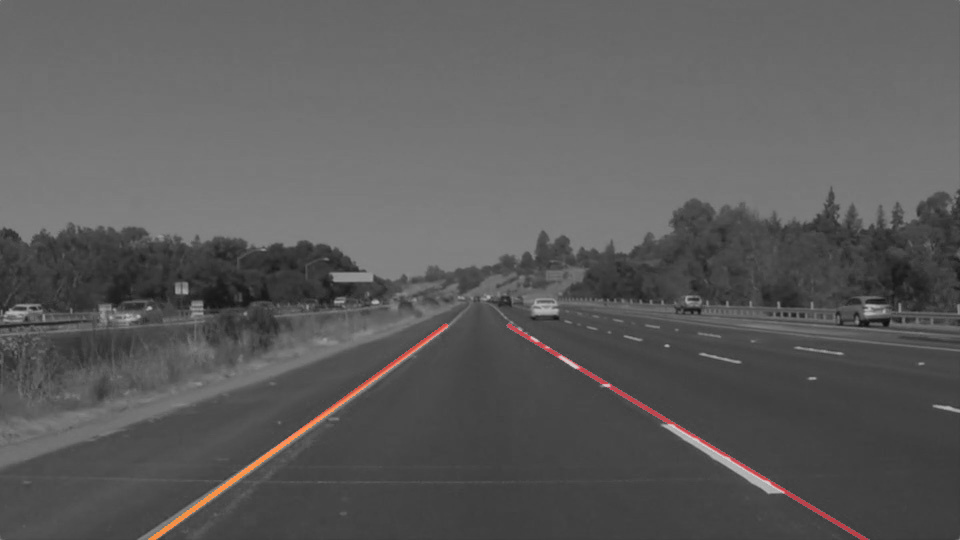
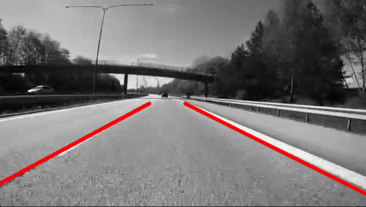
The algorithm can broken down into the following steps:
- Detect edges using the Canny edge detector.
- Extract the edges in the region of interest (a triangle covering the bottom corners and the center of the image).
- Run Hough transform to detect lanes.
车道线检测三步骤:
- 使用Canny边缘检测器检测边缘
- 提取图像中的感兴趣区域(图像中心的三角形区域)
- 使用霍夫变换检测车道线
2.1 Edge detection
Lanes on the roads are usually thin and long lines with bright colors. Our edge detection algorithm by itself should be able to find the lanes pretty well. Run the code cell below to load the example image and detect edges from the image.
1 | from edge import canny |

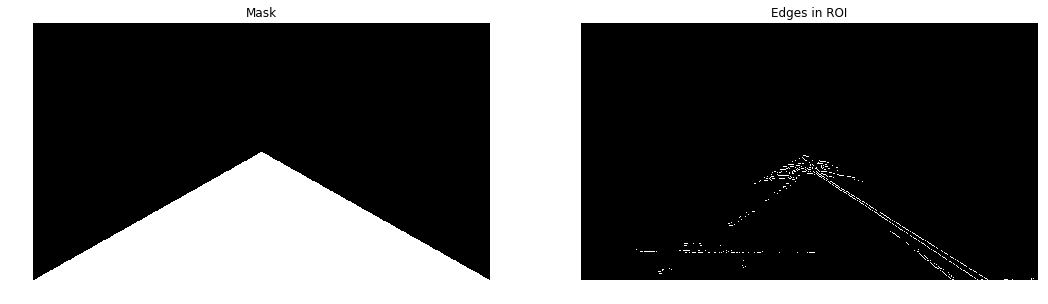
2.2 Extracting region of interest (ROI)
We can see that the Canny edge detector could find the edges of the lanes. However, we can also see that there are edges of other objects that we are not interested in. Given the position and orientation of the camera, we know that the lanes will be located in the lower half of the image. The code below defines a binary mask for the ROI and extract the edges within the region.
1 | H, W = img.shape |
2.3 Fitting lines using Hough transform (15 points)
The output from the edge detector is still a collection of connected points. However, it would be more natural to represent a lane as a line parameterized as $y = ax + b$, with a slope $a$ and y-intercept $b$. We will use Hough transform to find parameterized lines that represent the detected edges.
In general, a straight line $y = ax + b$ can be represented as a point $(a, b)$ in the parameter space. However, this cannot represent vertical lines as the slope parameter will be unbounded. Alternatively, we parameterize a line using $\theta\in{[-\pi, \pi]}$ and $\rho\in{\mathbb{R}}$ as follows:
$$
\rho = x\cdot{cos\theta} + y\cdot{sin\theta}
$$
Using this parameterization, we can map everypoint in $xy$-space to a sine-like line in $\theta\rho$-space (or Hough space). We then accumulate the parameterized points in the Hough space and choose points (in Hough space) with highest accumulated values. A point in Hough space then can be transformed back into a line in $xy$-space.
See notes on Hough transform.
Implement hough_transform in edge.py.
1 | from edge import hough_transform |
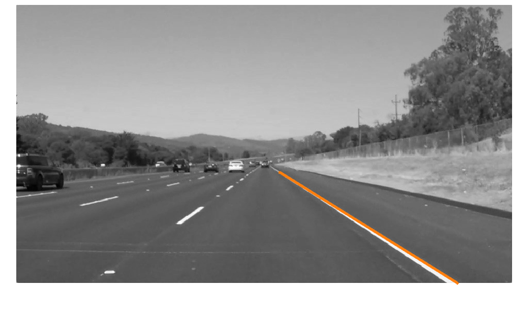
之所以只检测出一条直线,是因为上面的边缘检测部分不是很完美,尤其是左边车道线的边缘检测出现了问题,才会导致左边车道线做霍夫变换也得不到理想的结果。